How to use the Riparian Restoration to Promote Climate Change Resilience (RPCCR) Tool
by
Carol Sanders-Reed
—
last modified
Feb 23, 2024 02:44 PM
The following tutorial will describe the steps to depict the riparian areas that would benefit most from riparian restoration. The RPCCR tool enables users to dynamically locate areas (within the selected riparian zone region) that would benefit from increased shading produced by planting of trees. The tool operates on a 200 meter stream buffer (100 on each side), and requires the user to specify values for maximum percent canopy cover and minimum solar gain percentile. The user can additionally choose to include minimum elevation (meters) and maximum percent impervious surface values in the analysis.
RPCCR: How-to Instructional Exercise for General Users
Objective: The objective of this exercise is to familiarize you with the RPCCR and to assist each participant in utilizing the tool for a set of user-defined parameters.
Instructions:
- Access the Eastern Brook Trout Integrated Spatial data and Tools (EBTST) system: https://rpccr.ebtjv.de/ Chrome or Firefox browsers are preferred
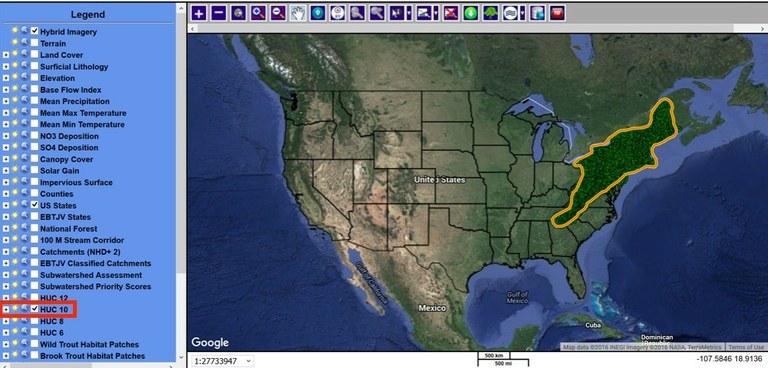
- Choose a HUC layer from the Legend check box list. The map will change, showing the HUC boundaries. For this example, select HUC 10.
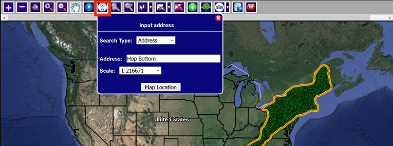
- Zoom to area of interest in order to select the polygon (or state) that you want to analyze. Click on the Zoom to Address tool and enter a location, either by name (Address) or by Coordinates. Example data has been provided for Tunkhannock Creek HUC 10 watershed (0205010612). To navigate to this area, search for Hop Bottom, Pennsylvania. Alternatively, you can manually navigate to the area of interest using the buttons on the upper-left hand section of the map window.
- Select the polygon (area) that you are interested in. First, you need to select the layer (HUC 10) by selecting the drop-down menu from the Select Features tool. The map will not change.
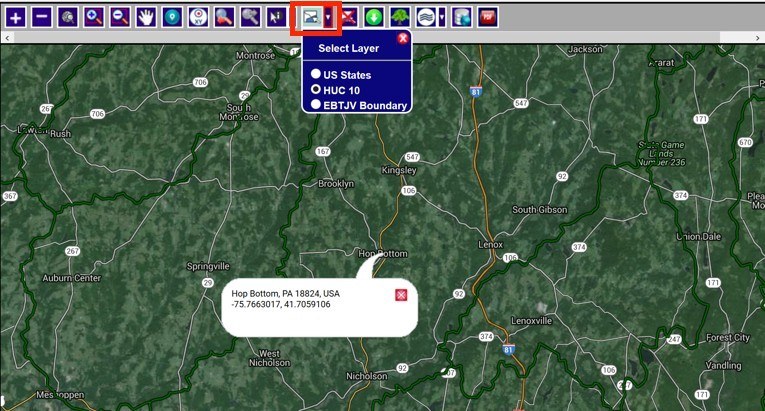
Then, click on the map in the HUC you are interested in. For this example, click near Hop Bottom, PA. The watershed of interest will be highlighted in blue. If you select the wrong HUC, click on the Clear Selected Features and then click in the watershed of interest.
If it takes more than 10 seconds to select the feature, you are probably trying to select the entire state. Refresh your browser and start again at step 2.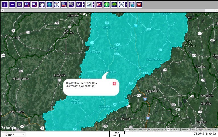
- Click on the RPCCR tool, which looks like a tree. Fill out the selection fields, including minimum canopy cover and maximum solar gain. A default value of 70 for % Canopy Cover and 75 for Solar Gain Percentile is automatically entered for these parameters, but this can be adjusted. The parameters for elevation and impervious surface are optional. To use these parameters in the analysis, click the check box to the left of those criteria and adjust the default values as necessary. Always select Restrict Extent by Selected Features; otherwise, the analysis will run for the entire Eastern Brook Trout area from Maine to Georgia. For this example, fill in the values in the box shown here.
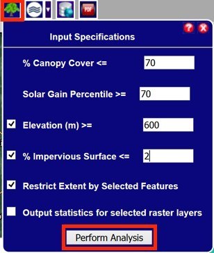
- Click Perform Analysis. After you click Perform Analysis, you will see the status bar listing the different steps and showing progress. When the analysis is complete, the status bar will disappear.
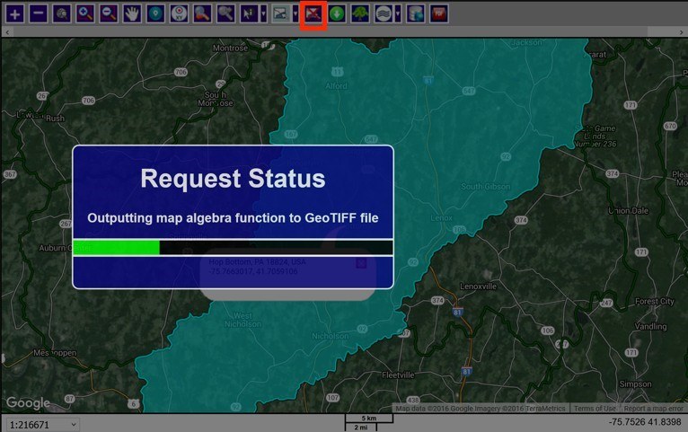
To see the RPCCR analysis, first remove the feature selection by clicking on the Clear Selected Features tool.
Note: The analysis can take some time to complete, especially for large areas such as a state. For one HUC the analysis should take less than a minute.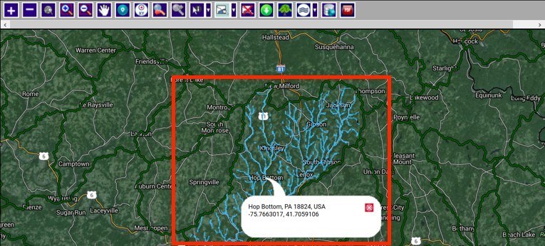
- Once the request is complete, all the riparian zones in the selected area will be displayed in light blue. The portions which match the selection criteria of canopy cover, solar gain, etc. will be displayed in dark blue.
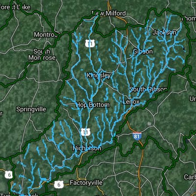
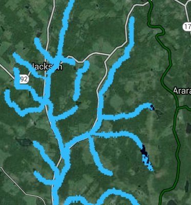
- The resulting layer is added to the list of layers that you can view to the left of the map. This new layer is at the bottom of the list.
- Each layer has a unique name listing the HUC fid and the selection criteria. For example, the name at the bottom of the list huc_10-680-70-70-600-2 was created by selecting area HUC 10 fid 680 with canopy cover less than 70% and solar gain of 70% or more with elevation of 600 and 2% Impervious surface.
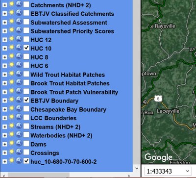
- Run the analysis several times with different parameter values to compare the results.
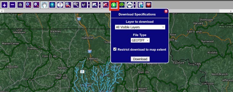
- Download the analysis results layer by clicking on Download tool. You can choose to download all the layers, or just the RPCCR analysis layer, which you will find by scrolling to the bottom of the All Visible Layers list. Choose GEOTIFF so that you can upload the layer to a GIS system.
